Overview
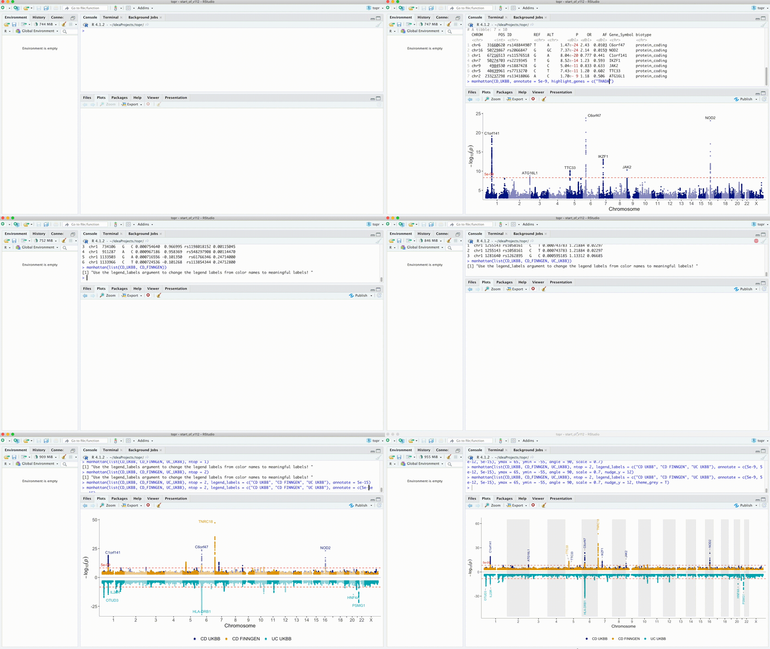
topr is a package for viewing and annotating genetic association results. See the GIF below for example functionality and visit the website for additional information and vignettes.

Click here to see the commands used in the .gif above
library(topr)

# Single GWAS manhattan plots
# Start by taking a look at one of topr's inbuilt datasets
CD_UKBB %>% head()
manhattan(CD_UKBB)
manhattan(CD_UKBB, annotate=5e-9)
CD_UKBB %>% get_lead_snps()
CD_UKBB %>% get_lead_snps() %>% annotate_with_nearest_gene()
manhattan(CD_UKBB, annotate=1e-9, highlight_genes=c("FTO","THADA"))
manhattan(CD_UKBB, annotate=1e-9, highlight_genes=c("FTO","THADA"), color="darkred")

# Multi GWAS manhattan/miami plots
CD_FINNGEN %>% head()
manhattan(list(CD_UKBB, CD_FINNGEN))
manhattan(list(CD_UKBB, CD_FINNGEN), legend_labels=c("UKBB","FINNGEN"))
manhattan(list(CD_UKBB, CD_FINNGEN), legend_labels=c("UKBB","FINNGEN"), ntop=1)


# Add the third GWAS result...
UC_UKBB %>% head()
manhattan(list(CD_UKBB, CD_FINNGEN, UC_UKBB))
manhattan(list(CD_UKBB, CD_FINNGEN, UC_UKBB), legend_labels=c("CD UKBB","CD FINNGEN", "UC UKBB"))
# display the first input dataset on the top plot (ntop = 1)
manhattan(list(CD_UKBB, CD_FINNGEN, UC_UKBB), legend_labels=c("CD UKBB","CD FINNGEN", "UC UKBB"), ntop=1)
# display the first TWO input datasets on the top plot (ntop = 2)
manhattan(list(CD_UKBB, CD_FINNGEN, UC_UKBB), legend_labels=c("CD UKBB","CD FINNGEN", "UC UKBB"), ntop=2)
manhattan(list(CD_UKBB, CD_FINNGEN, UC_UKBB), legend_labels=c("CD UKBB","CD FINNGEN", "UC UKBB"), ntop=2, annotate=1e-12)
#apply different annotation thresholds to the three datasets ( annotate = c(5e-9,1e-12,1e-15) )
manhattan(list(CD_UKBB, CD_FINNGEN, UC_UKBB), legend_labels=c("CD UKBB","CD FINNGEN", "UC UKBB"), ntop=2, annotate=c(5e-9,1e-12,1e-15))

# Make the plot look prettier by resetting they scales of the x and y  axes, changing the angle of the annotation text (angle = 90), moving it up a bit (nudge_y = 12) and slightly reducing the size of all text (scale = 0.7)
manhattan(list(CD_UKBB, CD_FINNGEN, UC_UKBB), legend_labels=c("CD UKBB","CD FINNGEN", "UC UKBB"), ntop=2, annotate=c(5e-9,1e-12,1e-15), ymax=65, ymin=-55, nudge_y=12,angle=90, scale=0.7)
# The same plot as above in the old topr grey theme (theme_grey = T)
manhattan(list(CD_UKBB, CD_FINNGEN, UC_UKBB), legend_labels=c("CD UKBB","CD FINNGEN", "UC UKBB"), ntop=2, annotate=c(5e-9,1e-12,1e-15), ymax=65, ymin=-55, nudge_y=12,angle=90, scale=0.7, theme_grey = T)
Citation
Please cite the following paper if you use topr in a publication:
Juliusdottir, T. topr: an R package for viewing and annotating genetic association results. BMC Bioinformatics 24, 268 (2023). https://doi.org/10.1186/s12859-023-05301-4
Installation
Install from CRAN:
install.packages("topr")Or from github:
devtools::install_github("totajuliusd/topr")And then load the package: